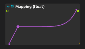
Mapping Curve

Create custom parameter mappings using an interactive curve editor. Draw curves to define exactly how input values should be transformed into output values, giving you precise control over parameter response characteristics.
Perfect for creating musical controller responses, sensor calibration curves, or any situation where you need non-linear parameter transformation that goes beyond simple linear scaling.
How it works
Mapping Curve presents a visual editor where you can draw or edit curves that define the relationship between input and output values. The X-axis represents input values (0-1), and the Y-axis represents output values (also 0-1 by default).
Input - Any control signal (0-1 range)
Curve editor - Interactive graphical curve editing
Output - Transformed value based on your curve
Curve types - Various curve shapes and mathematical functions
Curve editing features
Point editing: Click to add control points, drag to adjust curve shape, delete points to simplify curves.
Curve types: Linear segments, smooth curves, step functions, or mathematical curves like exponential, logarithmic, or sine waves.
Symmetry tools: Mirror curves horizontally or vertically for consistent response characteristics.
Preset curves: Common curves like exponential, logarithmic, S-curves, and inverse curves available as starting points.
Creative applications
Musical controllers: Shape MIDI controller response to feel more musical - make faders respond exponentially at low values, linearly in mid-range, and compress at high values.
Sensor calibration: Create custom calibration curves for sensors that don’t have linear responses - distance sensors, light sensors, or pressure sensors often need custom curves.
Expressive control: Design curves that provide fine control where you need it most - more sensitivity in certain ranges, less in others.
Audio parameter shaping: Create custom response curves for audio effect parameters - make filter cutoffs respond more naturally, or create special response characteristics for creative effects.
Visual effect timing: Shape animation curves for visual effects to create more natural or dramatic timing characteristics.
Advanced techniques
Multi-segment curves: Create complex curves with different characteristics in different ranges - linear at the bottom, exponential in the middle, compressed at the top.
Inverse curves: Create curves that invert normal parameter behavior for special effects or alternative control paradigms.
Asymmetric responses: Design curves that respond differently to increasing versus decreasing input values for unique interactive characteristics.
Micro-adjustments: Fine-tune specific regions of the curve for precise control over parameter behavior in critical ranges.
Integration with score
Mapping Curve works perfectly with any control source - MIDI controllers, sensor data from device protocols, LFO output, or any other parameter data that needs custom shaping.
Cascading curves: Chain multiple Mapping Curve processes for complex transformations that build on each other.
Parallel processing: Use multiple curves to create different parameter responses from the same input source.
Dynamic curves: While the curve shape is typically static, the input and output ranges can be controlled dynamically for evolving response characteristics.
Workflow tips
Start simple: Begin with basic exponential or logarithmic curves before creating complex multi-segment shapes.
Test thoroughly: Test your curves across the full input range to ensure they behave as expected in all conditions.
Consider context: Match your curve characteristics to the intended use - smooth curves for audio parameters, step functions for discrete control, exponential curves for natural-feeling responses.
Save presets: Save useful curves as presets for reuse in other projects or different parameters.
Common curve types
Exponential: Fast rise at the beginning, slower at the end - good for audio volume controls.
Logarithmic: Slow rise at the beginning, faster at the end - good for frequency controls.
S-curve: Slow at both ends, fast in the middle - good for natural-feeling responses.
Inverse: Flipped response characteristics - high input gives low output.
Step functions: Discrete jumps between values - useful for switching between preset values.
Related processes
Mapping Curve works with Mapping Tool for comprehensive parameter transformation, pairs with Calibrator for sensor work, and can shape the output of LFO or other control sources for more expressive parameter control.