Case study: scored air filtration in [re]capture

[re]capture (2022) is created by Alice Jarry and her team, consisting of Brice Ammar-Khodja, Jacqui Beaumont, Asa Perlman, Philippe Vandal, and Ariane Plante at Concordia University, where I am currently operating as a postdoctoral fellow.

This post presents a case study on the writing of a score with ossia score for such a complete artwork involving a wealth of interesting behaviours, sensors, actuators and protocols.

The [re]capture project

Exploring the concept of ‘filtration’ using biomaterials, plants, and electronic strategies, [re]capture is a dialogue between in situ atmospheric data capture devices and gallery installation. With air toxicity a growing issue, this ongoing project seeks to give shape to the microscopic invisibility and the macroscopic dimension of air pollution.

With the support of the Conseil des arts de Montréal, (@conseil.des.arts.de.montreal), the Fonds de recherche du Québec – Société et Culture (@fondsrecherchequebec) and the Concordia University Research Chair in Critical Practices in Materials and Materiality.

There are two main physical items involved in this artwork: air quality sensors (Nomad AirKits) which sense various atmospheric properties - temperature, CO² and pollution levels, etc., and the main installation which is a set of modules consisting of LEDs, fans and motors in a tubular circuit involving various materials, most importantly filtrating abaca and bioplastics. The general idea is that changes in sensor data will make the motors release dust in the tubular circuit ; fans will propel the dust inside it and LED lights accentuates the dramaturgy and allows the public to visualize the process.

To learn more about the artwork, head straight to the Materials Materiality research chair website

Prototyping and producing a score

The general idea for this score is still grounded in experimentation: the production time with the actual entire hardware set-up was a few days ; a big part of which was about learning how to play with the material and physical properties of the piece in order to make it look interesting.

This section will describe the setup, the general compositional process and the various features of score that were useful during the production work.

The goal is to leverage the external sensor data to activate the various air filtration modules inside the piece, by triggering motors and fans. For instance: when the CO² levels of a sensor reach some particular limit, something should happen ; the light intensity could be mapped to the average temperature of all the sensors ; etc. These mappings should evolve and vary over time to make the piece more dynamic.

Connecting ossia to the devices

Before doing anything, we have to focus on how score is going to interoperate with the external world for this piece: how are we going to get and process sensor data, and how are we going to control the stepper motors, LEDs, fans of the main installation.

There are as such two connections: inbound, from the sensors and outbound, to the serial port.

Input devices

The inbound connection is trivial: it is sufficient to create a new OSC device listening on the port on which the Nomad AirKits emit, and use the OSC learn functionality. The current experiment has three sets of sensors operating, simply identified as sensors:/<sensor number>/co2, etc.

Output devices

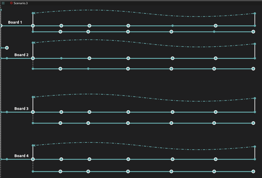
The outputs are controlled directly through a fairly simple serial protocol: the electronics side of the piece is divided in multiple boards. Each board has multiple controls. All the output modules are handled by this electronic board:

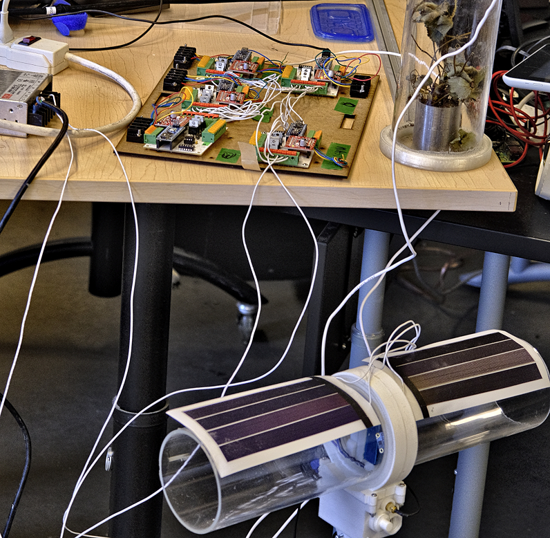
A Nomad AirKit is also pictured above: the tube with the small solar panel sheets.

Remember than score allows to communicate with arbitrary systems over a serial port thanks to the Serial device, which defines how the device tree maps to the actual communication protocol in QML / JS.

Here is the Serial device source code used for this work, which replaces a complex PureData patch.

import Ossia 1.0 as Ossia

Ossia.Serial {
    // The serial boards have a very low baud rate (56k). 
    // To not spam them too much, we force a coalescing 
    // of the values coming out of score so that there is 
    // at most one new value every 20 ms.    
    property real coalesce: 20

    // This is the implementation of the protocol our serial board expects: 
    // a b c \r \n
    // 
    // `a` is the board number byte
    // `b` is the control n° on that board
    // `c` the control value.
    // 
    // We use Uint8Array in order to send binary data.
    function frame(array)
    {
      let auint8 = new ArrayBuffer(5);
      let uint8 = new Uint8Array(auint8);
      uint8.set(array, 0);
      uint8[4] = '\r';
      uint8[5] = '\n';
      return auint8;
    }
    
    // Quick global mapping for our parameters.
    function mapValue(val, tp)
    {
        if(tp === 64)
        {
            // This is a bit of an emergency cheat we added to disable the stepper motors
            // in the central range as they were otherwise too noisy.
            if(val < (64 - 55)) return val;
            if(val > (64 + 55)) return val;
            return 64;
        }
        else
        {
            return val;
        }
    }

    // All our boards have the same parameters, so we refactor the parameter creation
    // with a simple utility function.
    function createNode(board)
    {
        // Each parameter is pretty similar so we can also refactor this.
        const createObj = (sensor, desc, def) => { return {
            name: sensor.toString(), 
            type: Ossia.Type.Int, 
            min: 0,
            max: 127,
            value: def,
            description: desc,
            request: (val) => frame([
                board + 128, 
                sensor, 
                mapValue(Math.max(Math.min(val.value, 127), 0), def)
            ])
        } };

        return { 
            name: board.toString(), 
            children: [
                  createObj(0, "stepper", 64)
                , createObj(5, "fet5", 0)
                , createObj(9, "fet9", 0)
            ] 
        };
    }

    // We have four boards, we define them here:
    function createTree() {
        let arr = [];
        for(let i = 1; i <= 4; i++)
          arr.push(createNode(i));
        return arr;
    }
}

Test cues

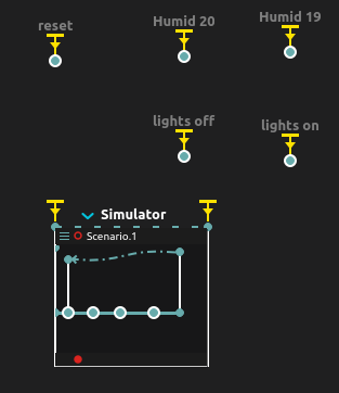
Sensors were not always available: some needed repairing, and their short battery life means that it was not possible to access live air pollution data at all times. To still be able to test changes in the score, a very simple pattern is to create a state (by double-clicking in the background of a scenario), drop the values of the cue from the explorer, set a trigger on it and mark it as enabled. It is also possible to make a small sub-scenario with a loop in order to have some automatic variation of our simulated sensor state.

Experimenting with mappings

Using the “local play” feature was instrumental for quick testing of individual mappings: at any point, it is possible to go inside a mapping sub-scenario and hit “Local play” (the “Play” button in orange, below): only this specific mapping will be executed, which allows to concentrate on making it look nice and interesting.

Organizing the score

For this score, we chose a triptych organisation. There are three “panels” in the score, which are going to loop over a hour and a half. Each gives a different perspective on the piece and involve different mappings with the sensors and actuators part of the piece.

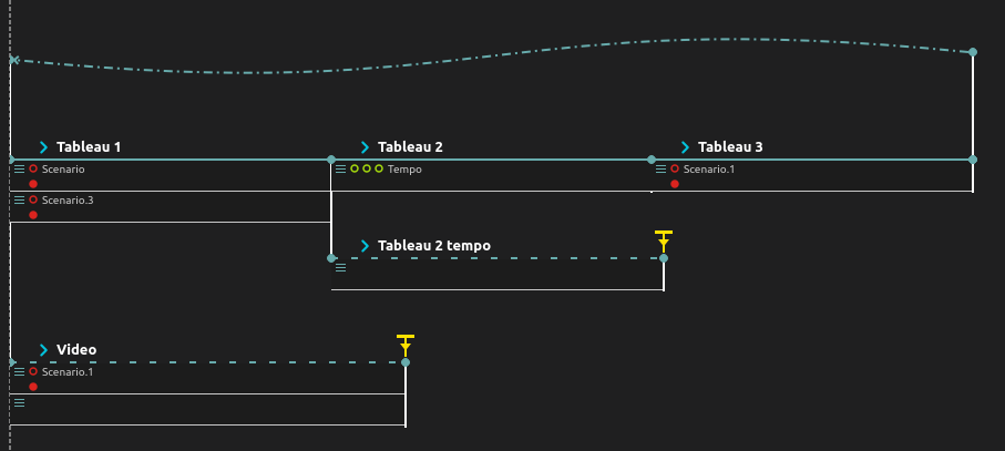
The first part contains individual mappings from sensors to modules. The second part is mainly pre-written automations, which are noisified and whose playback speed is altered depending on the external conditions. The last part is mappings from the average state of all the sensors, to all the modules taken together.

Making it loop

As you may know, it is fairly easy to make a score loop forever to run in installation mode, like this: it is done with the graph link, created by dragging from the small red plus icon when selecting the last state of the score.

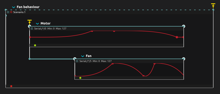
Score experiment: triggering a fan after a motor

One of the low-level scoring needs of the piece is that the fans should start blowing after the motors trigger in order to make sure that dust is indeed being blown in the tubes. Here’s a simple score example of how to do this:

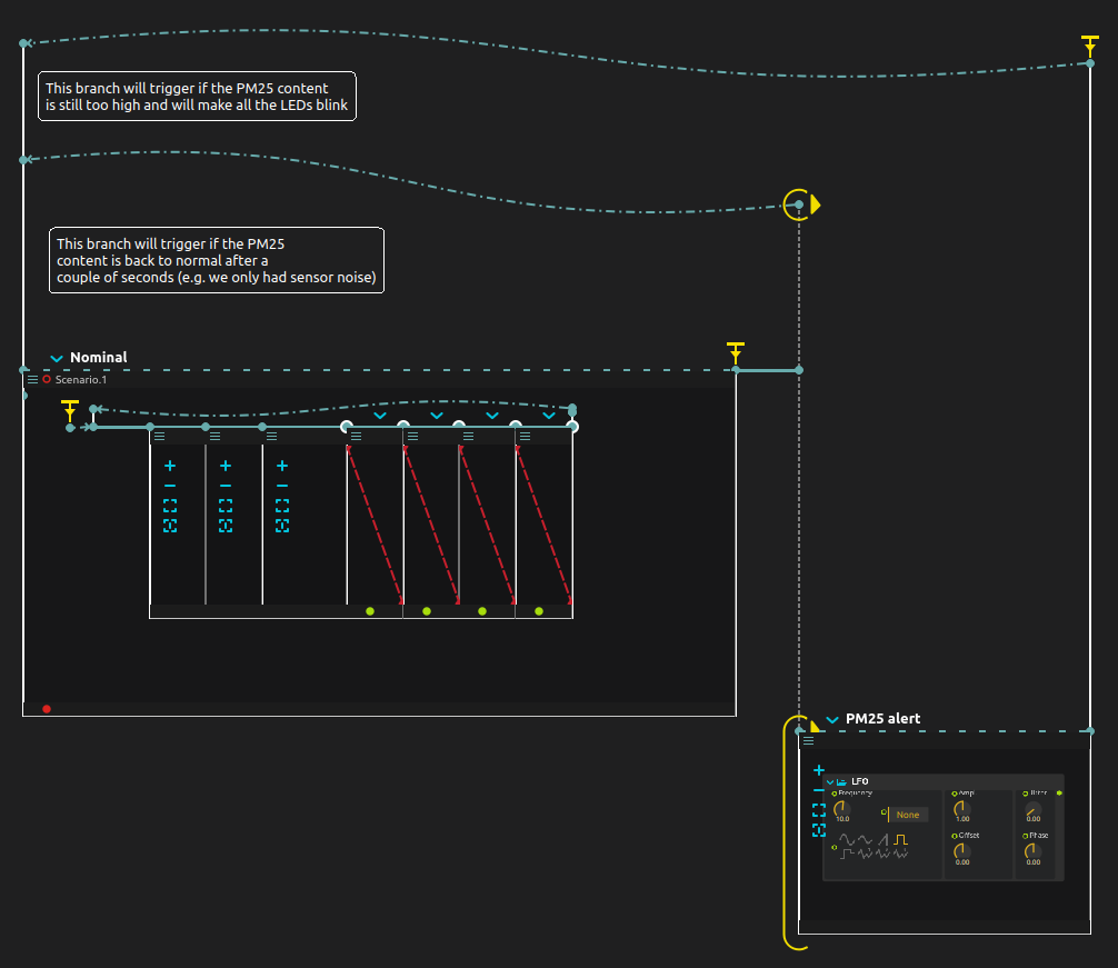
Score experiment: Emergency behaviours

One of the various ideas that were experimented with during the prototyping phase was to have a nominal behaviour for the piece, and switch to an “emergency” mode if for instance some sensor data is detected to be too high for human safety. The score shall go back to its nominal mode whenever the atmospheric particle levels go back to safer values.

Here is an example of a small score that implements this behaviour. This leverages all the syntax elements of the ossia score visual language: triggers, conditions, loop transitions…

Mappings

Mapping a set of sensor to a module

In this piece, we have as you remember:

• Sensors (Nomad AirKits). These are ESP32 boards which regularly send air quality and sensor data over OSC. The sensed parameters are: temperature, humidity, TVOC, CO², PM1, PM10, PM25.

• Modules: a module is a part of the installation which contains a LED ribbon, a stepper motor, and a fan to blow the dust inside the tubes.

The first approach for scoring, inspired from previous prototypes, has been to define a mapping / sub-score that processes arbitrary input sensors and writes it to an arbitrary module. In order to do this, we used a custom OSC device for storing score variables.

The composition rule for this part was that each mapping could leverage two distinct parameters, abstractly named “p1” and “p2” and map them to the three outputs of the module, stepper, led intensity and fan.

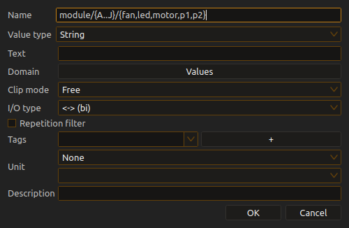
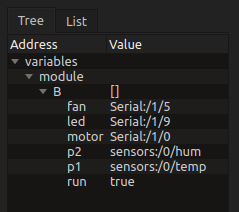
For this, we simply created a dummy OSC device which is used as a variables holder.

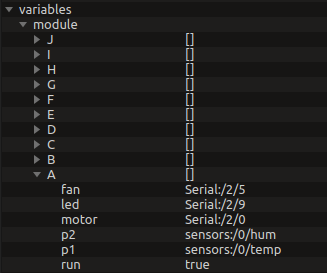
Creating such a device was actually fairly simple as it is possible to create multiple addresses thanks to OSC pattern expressions: the pattern module/{A..J}/{fan,led,motor,p1,p2} will automatically create most of the addresses needed in one go when entering the “Add child” dialog.

Then, we created our modules:

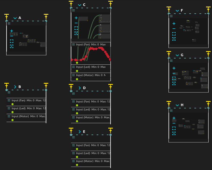
Each module has a slightly (or very) different behaviour. Some have pre-written parts for dramatic effect, while others are purely function of the input parameters. They are defined as free-floating intervals.

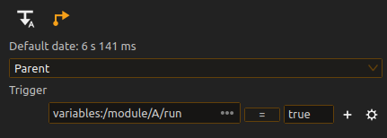
For each, the first trigger is configured to start whenever the OSC address variables:/modules/(the module)/run is set to true. Notice that “auto-play” is set on the trigger: otherwise, it will never start!

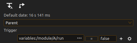
The last trigger is configured to kill the module when the run variable is set to false:

Then, inside each modules, the addresses are read live from the defined variables and used from the various objects in the mapping. For instance, the module A’s LED output is configured like this:

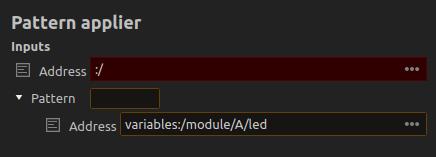
At runtime, whenever the address stored in variables:/modules/A/led changes (for instance it could be the string serial:/2/9, serial:/1/9 or even serial:/*/9 to address them all), the mapping’s output will be redirected to the new parameter.

Finally, we have a small temporal composition of states which will change the value of these variables over time ; the score is organised per-module board, that is, the first line defines all the modules used by the module 1, etc.:

Each state will change the module used at a given point in time by a board ; it looks like this:

This of course calls for some evolutions to ossia score to make this kind of compositional system easier to define and write for: mainly, we are missing the ability to instantiate and remove a given module on the fly and use them as a template.

Scripting

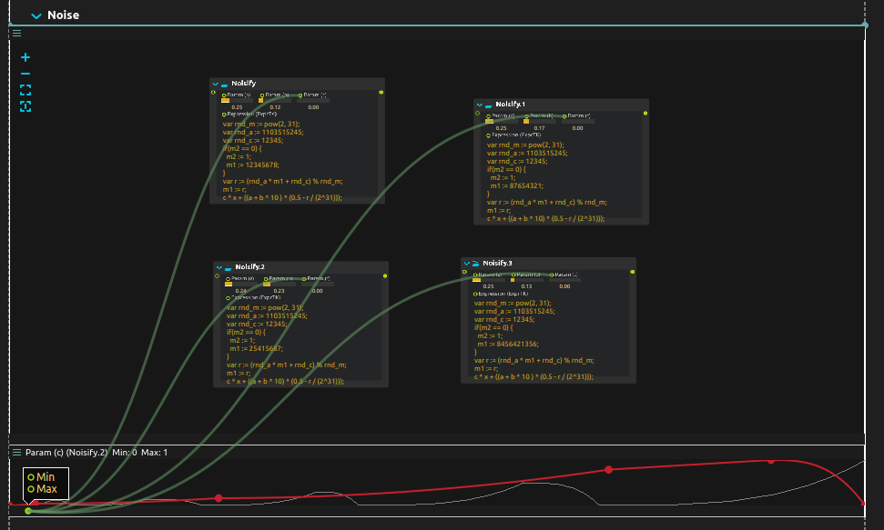
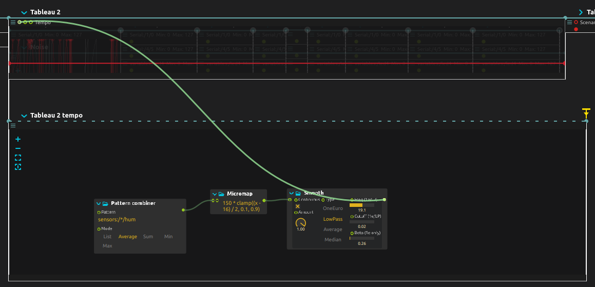
The second part of the score uses another approach: the general shape of the parameter evolutions for every module is written manually, in order to try to emphasis a slightly more dramatic narrative that the one we are able to achieve with simple parameter mapping.

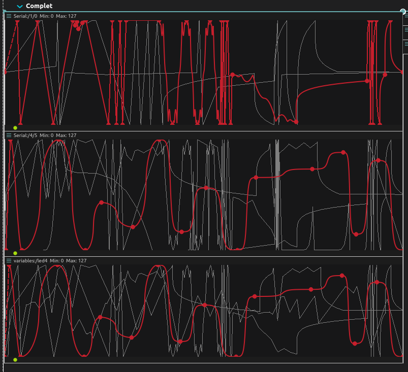
The LED automations are not directly used to control the LEDs ; before, they go through an expression mapper which adds progressively more noise both over time and depending on the external conditions detected by the sensors.

Finally, we also use an average humidity measure to control the speed at which these automations are being played, by using a tempo process and writing a small mapping. In many parts of the score, the Smooth object was extremely useful: the sensors only give updated values every 5-10 seconds on average, which would sometimes give very surprising jumps. Smoothing over a second-ish allows to avoid that.

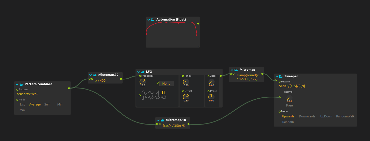
Global mappings

Finally, the last part of our tryptich focuses on mapping averages of our sensor data into communicating behaviour across all the modules. For this, we used for instance the Sweeper object described below, which makes a specific behaviour “run” across all the serial modules in a rhythm defined by one of the sensor data. Multiple mappings succeed one another. Below, one is pictured: it maps the CO² average of our sensors to both light intensity and circulation speed of the LEDs and fans.

Video mapping

The piece also features a video projection of video recordings done at the sites where the Nomad Airkits did air measurements. The video feed, captured with a 360° fisheye camera, is re-projected on the artwork.

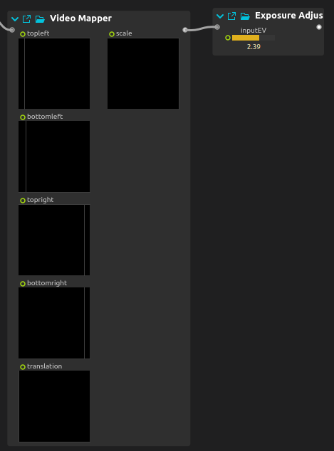
On squishiness and light adjustements

The video projection used made the video too wide: we used a very quick and dirty Video Mapper object to make it more round to fit the artwork. Likewise, some exposure adjust was needed as the video projector we had really wasn’t bright enough. Thankfully, ossia score’s user library comes with objects for handling this built-in, thanks to the great ISF library shared by Vidvox!

Mapping parameters to real-time video filters

In addition, we can of course use parameters from our sensors to adjust the video. For this experiment, we simply mapped the measured temperature to the chromaticity of the displayed picture ; more interesting mappings could very likely be devised over time.

New objects for pattern control

As part of the conception of this artwork, a few new objects made their way into score, which can be generally useful to the community. They could be developed very quickly thanks to the magical superpowers of Avendish which makes writing custom ossia objects an absolute breeze ; the development time for each object was at most one hour for each.

Here’s an overview:

Calibrator

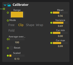
This object was born from the observation that every sensor would have a fairly different range depending on the time of the day. It calibrates the input signal with its actual min and max bound over time, in order to enable to detect meaningful variations in the signal. It also provides some useful statistical analysis tools: mean, variance, lower and upper bound.

It is available under Control > Mappings in the processes pane.

Pattern combiner

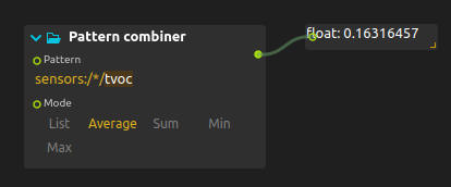
This object fetches and processes addresses matching an OSC pattern, and allows to compute for instance the mean of the matched parameters, combine them in a list, etc.

Note that if you just need to get all the messages in succession from a set of OSC addresses, no particular object is needed: you can just directly use a pattern match expression as the input of a port in the address field.

It is available under Control > Data Processing in the processes pane.

Pattern applier

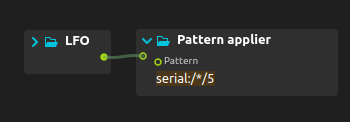
This object takes a list as input, and an address pattern for output which will match multiple addresses.

For instance: if the pattern is serial:/*/5, the actual addresses will be in our case serial:/1/5, serial:/2/5, serial:/3/5 , serial:/4/5.

The object will send every element of the list passed in input to the addresses, e.g. if the list [4, 6, 12, 7] is passed as input to the object, then serial:/1/5 will get 4, serial:/2/5 will get 6, serial:/3/5 will get 12, etc.

It is available under Control > Data Processing in the processes pane.

Note that if you need to send the same message to every address matching a pattern, no specific object is needed: OSC pattern match expressions can already be specified for every output port of score.

Pattern sweeper

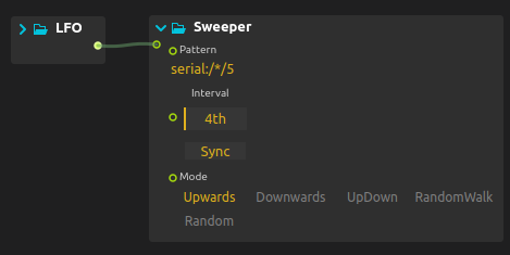
This object sweeps over the addresses specified in the pattern expression at a given rhythm.

For instance, in the screenshot below, every quarter note, the next address matched by the pattern will get the input routed to it.

It is available under Control > Data Processing in the processes pane.

Conclusion

Thanks for reading all this! In the end, I must say that I had a lot of fun writing the score for this piece ; it also brought some small usability issues to the spotlight, which will be worked on in further releases.